Calculating and Visualizing Sequence Statistics
This example shows how to use basic sequence manipulation techniques and computes some useful sequence statistics. It also illustrates how to look for coding regions (such as proteins) and pursue further analysis of them.
The Human Mitochondrial Genome
In this example you will explore the DNA sequence of the human mitochondria. Mitochondria are structures, called organelles, that are found in the cytoplasm of the cell in hundreds to thousands for each cell. Mitochondria are generally the major energy production center in eukaryotes, they help to degrade fats and sugars.
The consensus sequence of the human mitochondria genome has accession number NC_012920. You can getgenbank function to get the latest annotated sequence from GenBank® into the MATLAB® workspace.
mitochondria_gbk = getgenbank('NC_012920');
For your convenience, previously downloaded sequence is included in a MAT-file. Note that data in public repositories is frequently curated and updated; therefore the results of this example might be slightly different when you use up-to-date datasets.
load mitochondria
Copy just the DNA sequence to a new variable mitochondria. You can access parts of the DNA sequence by using regular MATLAB indexing commands.
mitochondria = mitochondria_gbk.Sequence;
mitochondria_length = length(mitochondria)
first_300_bases = seqdisp(mitochondria(1:300))
mitochondria_length =

       16569


first_300_bases =

  5×70 char array

    '  1  GATCACAGGT CTATCACCCT ATTAACCACT CACGGGAGCT CTCCATGCAT TTGGTATTTT'
    ' 61  CGTCTGGGGG GTATGCACGC GATAGCATTG CGAGACGCTG GAGCCGGAGC ACCCTATGTC'
    '121  GCAGTATCTG TCTTTGATTC CTGCCTCATC CTATTATTTA TCGCACCTAC GTTCAATATT'
    '181  ACAGGCGAAC ATACTTACTA AAGTGTGTTA ATTAATTAAT GCTTGTAGGA CATAATAATA'
    '241  ACAATTGAAT GTCTGCACAG CCACTTTCCA CACAGACATC ATAACAAAAA ATTTCCACCA'
You can look at the composition of the nucleotides with the ntdensity function.
figure
ntdensity(mitochondria)
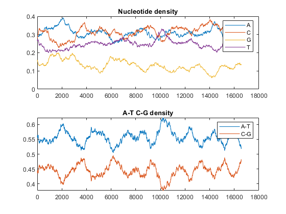
This shows that the mitochondria genome is A-T rich. The GC-content is sometimes used to classify organisms in taxonomy, it may vary between different species from ~30% up to ~70%. Measuring GC content is also useful for identifying genes and for estimating the annealing temperature of DNA sequence.
Calculating Sequence Statistics
Now, you will use some of the sequence statistics functions in the Bioinformatics Toolbox™ to look at various properties of the human mitochondrial genome. You can count the number of bases of the whole sequence using the basecount function.
bases = basecount(mitochondria)
bases =

  struct with fields:

    A: 5124
    C: 5181
    G: 2169
    T: 4094
These are on the 5'-3' strand. You can look at the reverse complement case using the seqrcomplement function.
compBases = basecount(seqrcomplement(mitochondria))
compBases =

  struct with fields:

    A: 4094
    C: 2169
    G: 5181
    T: 5124
As expected, the base counts on the reverse complement strand are complementary to the counts on the 5'-3' strand.
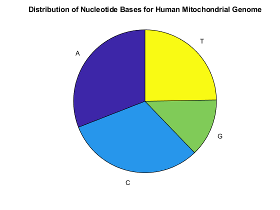
You can use the chart option to basecount to display a pie chart of the distribution of the bases.
figure
basecount(mitochondria,'chart','pie');
title('Distribution of Nucleotide Bases for Human Mitochondrial Genome');
Now look at the dimers in the sequence and display the information in a bar chart using dimercount.
figure
dimers = dimercount(mitochondria,'chart','bar')
title('Mitochondrial Genome Dimer Histogram');
dimers =

  struct with fields:

    AA: 1604
    AC: 1495
    AG: 795
    AT: 1230
    CA: 1534
    CC: 1771
    CG: 435
    CT: 1440
    GA: 613
    GC: 711
    GG: 425
    GT: 419
    TA: 1373
    TC: 1204
    TG: 513
    TT: 1004

Exploring the Open Reading Frames (ORFs)
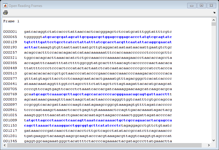
In a nucleotide sequence an obvious thing to look for is if there are any open reading frames. An ORF is any sequence of DNA or RNA that can be potentially translated into a protein. The function seqshoworfs can be used to visualize ORFs in a sequence.
Note: In the HTML tutorial only the first page of the output is shown, however when running the example you will be able to inspect the complete mitochondrial genome using the scrollbar on the figure.
seqshoworfs(mitochondria);
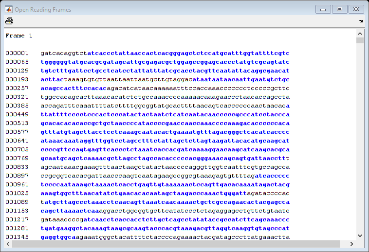
If you compare this output to the genes shown on the NCBI page there seem to be slightly fewer ORFs, and hence fewer genes, than expected.
Vertebrate mitochondria do not use the Standard genetic code so some codons have different meaning in mitochondrial genomes. For more information about using different genetic codes in MATLAB see the help for the function geneticcode. The GeneticCode option to the seqshoworfs function allows you to look at the ORFs again but this time with the vertebrate mitochondrial genetic code.
In the human mitochondrial DNA sequence some genes are also started by alternative start codons [1]. Use the AlternativeStartCodons option to the seqshoworfs function to search also for these ORFs.
Notice that there are now two much larger ORFs on the third reading frame: One starting at position 4470 and the other starting at 5904. These correspond to the ND2 (NADH dehydrogenase subunit 2) and COX1 (cytochrome c oxidase subunit I) genes.
orfs = seqshoworfs(mitochondria,'GeneticCode','Vertebrate Mitochondrial',...
        'AlternativeStartCodons',true)
orfs =

  1×3 struct array with fields:

    Start
    Stop
Inspecting Annotated Features
You can also look at all the features that have been annotated to the human mitochondrial genome. Explore the complete GenBank entry mitochondria_gbk with the featureparse function. Particularly, you can explore the annotated coding sequences (CDS) and compare them with the ORFs previously found. Use the Sequence option to the featureparse function to extract, when possible, the DNA sequences respective to each feature. The featureparse function will complement the pieces of the source sequence when appropriate.
features = featureparse(mitochondria_gbk,'Sequence',true)
coding_sequences = features.CDS;
coding_sequences_id = sprintf('%s ',coding_sequences.gene)
features =

  struct with fields:

          source: [1×1 struct]
          D_loop: [1×1 struct]
            gene: [1×37 struct]
            tRNA: [1×22 struct]
            rRNA: [1×2 struct]
             STS: [1×28 struct]
    misc_feature: [1×1 struct]
             CDS: [1×13 struct]


coding_sequences_id =

    'ND1 ND2 COX1 COX2 ATP8 ATP6 COX3 ND3 ND4L ND4 ND5 ND6 CYTB '
ND2CDS = coding_sequences(2) % ND2 is in the 2nd position
COX1CDS = coding_sequences(3) % COX1 is in the 3rd position
ND2CDS =

  struct with fields:

         Location: '4470..5511'
          Indices: [4470 5511]
             gene: 'ND2'
     gene_synonym: 'MTND2'
             note: 'TAA stop codon is completed by the addition of 3' A residues to the mRNA'
      codon_start: '1'
    transl_except: '(pos:5511,aa:TERM)'
     transl_table: '2'
          product: 'NADH dehydrogenase subunit 2'
       protein_id: 'YP_003024027.1'
          db_xref: {'GI:251831108'  'GeneID:4536'  'HGNC:7456'  'MIM:516001'}
      translation: 'MNPLAQPVIYSTIFAGTLITALSSHWFFTWVGLEMNMLAFIPVLTKKMNPRSTEAAIKYFLTQATASMILLMAILFNNMLSGQWTMTNTTNQYSSLMIMMAMAMKLGMAPFHFWVPEVTQGTPLTSGLLLLTWQKLAPISIMYQISPSLNVSLLLTLSILSIMAGSWGGLNQTQLRKILAYSSITHMGWMMAVLPYNPNMTILNLTIYIILTTTAFLLLNLNSSTTTLLLSRTWNKLTWLTPLIPSTLLSLGGLPPLTGFLPKWAIIEEFTKNNSLIIPTIMATITLLNLYFYLRLIYSTSITLLPMSNNVKMKWQFEHTKPTPFLPTLIALTTLLLPISPFMLMIL'
         Sequence: 'attaatcccctggcccaacccgtcatctactctaccatctttgcaggcacactcatcacagcgctaagctcgcactgattttttacctgagtaggcctagaaataaacatgctagcttttattccagttctaaccaaaaaaataaaccctcgttccacagaagctgccatcaagtatttcctcacgcaagcaaccgcatccataatccttctaatagctatcctcttcaacaatatactctccggacaatgaaccataaccaatactaccaatcaatactcatcattaataatcataatagctatagcaataaaactaggaatagccccctttcacttctgagtcccagaggttacccaaggcacccctctgacatccggcctgcttcttctcacatgacaaaaactagcccccatctcaatcatataccaaatctctccctcactaaacgtaagccttctcctcactctctcaatcttatccatcatagcaggcagttgaggtggattaaaccaaacccagctacgcaaaatcttagcatactcctcaattacccacataggatgaataatagcagttctaccgtacaaccctaacataaccattcttaatttaactatttatattatcctaactactaccgcattcctactactcaacttaaactccagcaccacgaccctactactatctcgcacctgaaacaagctaacatgactaacacccttaattccatccaccctcctctccctaggaggcctgcccccgctaaccggctttttgcccaaatgggccattatcgaagaattcacaaaaaacaatagcctcatcatccccaccatcatagccaccatcaccctccttaacctctacttctacctacgcctaatctactccacctcaatcacactactccccatatctaacaacgtaaaaataaaatgacagtttgaacatacaaaacccaccccattcctccccacactcatcgcccttaccacgctactcctacctatctccccttttatactaataatcttat'


COX1CDS =

  struct with fields:

         Location: '5904..7445'
          Indices: [5904 7445]
             gene: 'COX1'
     gene_synonym: 'COI; MTCO1'
             note: 'cytochrome c oxidase I'
      codon_start: '1'
    transl_except: []
     transl_table: '2'
          product: 'cytochrome c oxidase subunit I'
       protein_id: 'YP_003024028.1'
          db_xref: {'GI:251831109'  'GeneID:4512'  'HGNC:7419'  'MIM:516030'}
      translation: 'MFADRWLFSTNHKDIGTLYLLFGAWAGVLGTALSLLIRAELGQPGNLLGNDHIYNVIVTAHAFVMIFFMVMPIMIGGFGNWLVPLMIGAPDMAFPRMNNMSFWLLPPSLLLLLASAMVEAGAGTGWTVYPPLAGNYSHPGASVDLTIFSLHLAGVSSILGAINFITTIINMKPPAMTQYQTPLFVWSVLITAVLLLLSLPVLAAGITMLLTDRNLNTTFFDPAGGGDPILYQHLFWFFGHPEVYILILPGFGMISHIVTYYSGKKEPFGYMGMVWAMMSIGFLGFIVWAHHMFTVGMDVDTRAYFTSATMIIAIPTGVKVFSWLATLHGSNMKWSAAVLWALGFIFLFTVGGLTGIVLANSSLDIVLHDTYYVVAHFHYVLSMGAVFAIMGGFIHWFPLFSGYTLDQTYAKIHFTIMFIGVNLTFFPQHFLGLSGMPRRYSDYPDAYTTWNILSSVGSFISLTAVMLMIFMIWEAFASKRKVLMVEEPSMNLEWLYGCPPPYHTFEEPVYMKS'
         Sequence: 'atgttcgccgaccgttgactattctctacaaaccacaaagacattggaacactatacctattattcggcgcatgagctggagtcctaggcacagctctaagcctccttattcgagccgagctgggccagccaggcaaccttctaggtaacgaccacatctacaacgttatcgtcacagcccatgcatttgtaataatcttcttcatagtaatacccatcataatcggaggctttggcaactgactagttcccctaataatcggtgcccccgatatggcgtttccccgcataaacaacataagcttctgactcttacctccctctctcctactcctgctcgcatctgctatagtggaggccggagcaggaacaggttgaacagtctaccctcccttagcagggaactactcccaccctggagcctccgtagacctaaccatcttctccttacacctagcaggtgtctcctctatcttaggggccatcaatttcatcacaacaattatcaatataaaaccccctgccataacccaataccaaacgcccctcttcgtctgatccgtcctaatcacagcagtcctacttctcctatctctcccagtcctagctgctggcatcactatactactaacagaccgcaacctcaacaccaccttcttcgaccccgccggaggaggagaccccattctataccaacacctattctgatttttcggtcaccctgaagtttatattcttatcctaccaggcttcggaataatctcccatattgtaacttactactccggaaaaaaagaaccatttggatacataggtatggtctgagctatgatatcaattggcttcctagggtttatcgtgtgagcacaccatatatttacagtaggaatagacgtagacacacgagcatatttcacctccgctaccataatcatcgctatccccaccggcgtcaaagtatttagctgactcgccacactccacggaagcaatatgaaatgatctgctgcagtgctctgagccctaggattcatctttcttttcaccgtaggtggcctgactggcattgtattagcaaactcatcactagacatcgtactacacgacacgtactacgttgtagcccacttccactatgtcctatcaataggagctgtatttgccatcataggaggcttcattcactgatttcccctattctcaggctacaccctagaccaaacctacgccaaaatccatttcactatcatattcatcggcgtaaatctaactttcttcccacaacactttctcggcctatccggaatgccccgacgttactcggactaccccgatgcatacaccacatgaaacatcctatcatctgtaggctcattcatttctctaacagcagtaatattaataattttcatgatttgagaagccttcgcttcgaagcgaaaagtcctaatagtagaagaaccctccataaacctggagtgactatatggatgccccccaccctaccacacattcgaagaacccgtatacataaaatctaga'
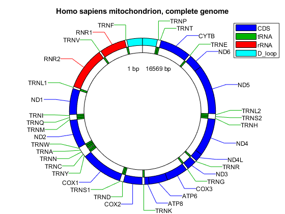
Create a map indicating all the features found in this GenBank entry using the featureview function.
[h,l] = featureview(mitochondria_gbk,{'CDS','tRNA','rRNA','D_loop'},...
                                      [2 1 2 2 2],'Fontsize',9);
legend(h,l,'interpreter','none');
title('Homo sapiens mitochondrion, complete genome')
Extracting and Analyzing the ND2 and COX1 Proteins
You can translate the DNA sequences that code for the ND2 and COX1 proteins by using the nt2aa function. Again the GeneticCode option must be used to specify the vertebrate mitochondrial genetic code.
ND2 = nt2aa(ND2CDS,'GeneticCode','Vertebrate Mitochondrial');
disp(seqdisp(ND2))
  1  MNPLAQPVIY STIFAGTLIT ALSSHWFFTW VGLEMNMLAF IPVLTKKMNP RSTEAAIKYF
 61  LTQATASMIL LMAILFNNML SGQWTMTNTT NQYSSLMIMM AMAMKLGMAP FHFWVPEVTQ
121  GTPLTSGLLL LTWQKLAPIS IMYQISPSLN VSLLLTLSIL SIMAGSWGGL NQTQLRKILA
181  YSSITHMGWM MAVLPYNPNM TILNLTIYII LTTTAFLLLN LNSSTTTLLL SRTWNKLTWL
241  TPLIPSTLLS LGGLPPLTGF LPKWAIIEEF TKNNSLIIPT IMATITLLNL YFYLRLIYST
301  SITLLPMSNN VKMKWQFEHT KPTPFLPTLI ALTTLLLPIS PFMLMIL
COX1 = nt2aa(COX1CDS,'GeneticCode','Vertebrate Mitochondrial');
disp(seqdisp(COX1))
  1  MFADRWLFST NHKDIGTLYL LFGAWAGVLG TALSLLIRAE LGQPGNLLGN DHIYNVIVTA
 61  HAFVMIFFMV MPIMIGGFGN WLVPLMIGAP DMAFPRMNNM SFWLLPPSLL LLLASAMVEA
121  GAGTGWTVYP PLAGNYSHPG ASVDLTIFSL HLAGVSSILG AINFITTIIN MKPPAMTQYQ
181  TPLFVWSVLI TAVLLLLSLP VLAAGITMLL TDRNLNTTFF DPAGGGDPIL YQHLFWFFGH
241  PEVYILILPG FGMISHIVTY YSGKKEPFGY MGMVWAMMSI GFLGFIVWAH HMFTVGMDVD
301  TRAYFTSATM IIAIPTGVKV FSWLATLHGS NMKWSAAVLW ALGFIFLFTV GGLTGIVLAN
361  SSLDIVLHDT YYVVAHFHYV LSMGAVFAIM GGFIHWFPLF SGYTLDQTYA KIHFTIMFIG
421  VNLTFFPQHF LGLSGMPRRY SDYPDAYTTW NILSSVGSFI SLTAVMLMIF MIWEAFASKR
481  KVLMVEEPSM NLEWLYGCPP PYHTFEEPVY MKS*
You can get a more complete picture of the amino acid content with aacount.
figure
subplot(2,1,1)
ND2aaCount = aacount(ND2,'chart','bar');
title('Histogram of Amino Acid Count for the ND2 Protein');

subplot(2,1,2)
COX1aaCount = aacount(COX1,'chart','bar');
title('Histogram of Amino Acid Count for the COX1 Protein');
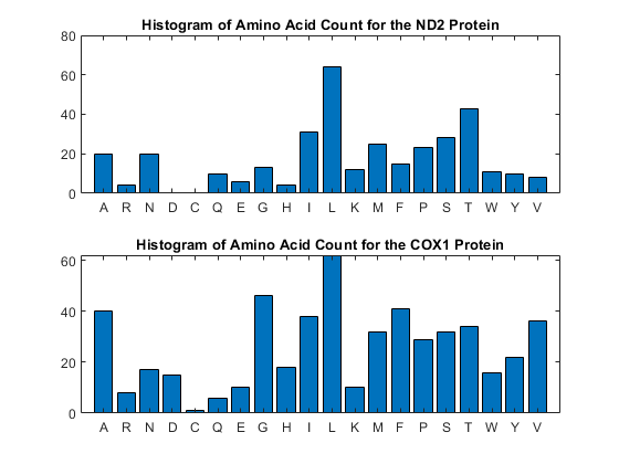
Notice the high leucine, threonine and isoleucine content and also the lack of cysteine or aspartic acid.
You can use the atomiccomp and molweight functions to calculate more properties about the ND2 protein.
ND2AtomicComp = atomiccomp(ND2)
ND2MolWeight = molweight(ND2)
ND2AtomicComp =

  struct with fields:

    C: 1818
    H: 2882
    N: 420
    O: 471
    S: 25


ND2MolWeight =

   3.8960e+04
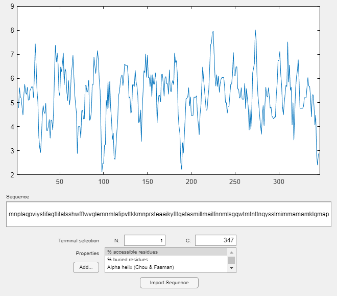
For further investigation of the properties of the ND2 protein, use proteinplot. This is a graphical user interface (GUI) that allows you to easily create plots of various properties, such as hydrophobicity, of a protein sequence. Click on the "Edit" menu to create new properties, to modify existing property values, or, to adjust the smoothing parameters. Click on the "Help" menu in the GUI for more information on how to use the tool.
proteinplot(ND2)
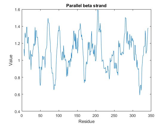
You can also programmatically create plots of various properties of the sequence using proteinpropplot.
figure
proteinpropplot(ND2,'PropertyTitle','Parallel beta strand')
Calculating the Codon Frequency using all the Genes in the Human Mitochondrial Genome
The codoncount function counts the number of occurrences of each codon in the sequence and displays a formatted table of the result.
codoncount(ND2CDS)
AAA - 10     AAC - 14     AAG -  2     AAT -  6
ACA - 11     ACC - 24     ACG -  3     ACT -  5
AGA -  0     AGC -  4     AGG -  0     AGT -  1
ATA - 23     ATC - 24     ATG -  1     ATT -  8
CAA -  8     CAC -  3     CAG -  2     CAT -  1
CCA -  4     CCC - 12     CCG -  2     CCT -  5
CGA -  0     CGC -  3     CGG -  0     CGT -  1
CTA - 26     CTC - 18     CTG -  4     CTT -  7
GAA -  5     GAC -  0     GAG -  1     GAT -  0
GCA -  8     GCC -  7     GCG -  1     GCT -  4
GGA -  5     GGC -  7     GGG -  0     GGT -  1
GTA -  3     GTC -  2     GTG -  0     GTT -  3
TAA -  0     TAC -  8     TAG -  0     TAT -  2
TCA -  7     TCC - 11     TCG -  1     TCT -  4
TGA - 10     TGC -  0     TGG -  1     TGT -  0
TTA -  8     TTC -  7     TTG -  1     TTT -  8
Notice that in the ND2 gene there are more CTA, ATC and ACC codons than others. You can check what amino acids these codons get translated into using the nt2aa and aminolookup functions.
CTA_aa = aminolookup('code',nt2aa('CTA'))
ATC_aa = aminolookup('code',nt2aa('ATC'))
ACC_aa = aminolookup('code',nt2aa('ACC'))
CTA_aa =

    'Leu	Leucine
     '


ATC_aa =

    'Ile	Isoleucine
     '


ACC_aa =

    'Thr	Threonine
     '
To calculate the codon frequency for all the genes you can concatenate them into a single sequence before using the function codoncount. You need to ensure that the codons are complete (three nucleotides each) so the read frame of the sequence is not lost at the concatenation.
numCDS = numel(coding_sequences);
CDS = cell(numCDS,1);
for i = 1:numCDS
     seq = coding_sequences(i).Sequence;
     CDS{i} = seq(1:3*floor(length(seq)/3));
end
allCDS = [CDS{:}];
codoncount(allCDS)
AAA -  85     AAC - 132     AAG -  10     AAT -  32
ACA - 134     ACC - 155     ACG -  10     ACT -  52
AGA -   1     AGC -  39     AGG -   1     AGT -  14
ATA - 167     ATC - 196     ATG -  40     ATT - 124
CAA -  82     CAC -  79     CAG -   8     CAT -  18
CCA -  52     CCC - 119     CCG -   7     CCT -  41
CGA -  28     CGC -  26     CGG -   2     CGT -   7
CTA - 276     CTC - 167     CTG -  45     CTT -  65
GAA -  64     GAC -  51     GAG -  24     GAT -  15
GCA -  80     GCC - 124     GCG -   8     GCT -  43
GGA -  67     GGC -  87     GGG -  34     GGT -  24
GTA -  70     GTC -  48     GTG -  18     GTT -  31
TAA -   3     TAC -  89     TAG -   2     TAT -  46
TCA -  83     TCC -  99     TCG -   7     TCT -  32
TGA -  93     TGC -  17     TGG -  11     TGT -   5
TTA -  73     TTC - 139     TTG -  18     TTT -  77
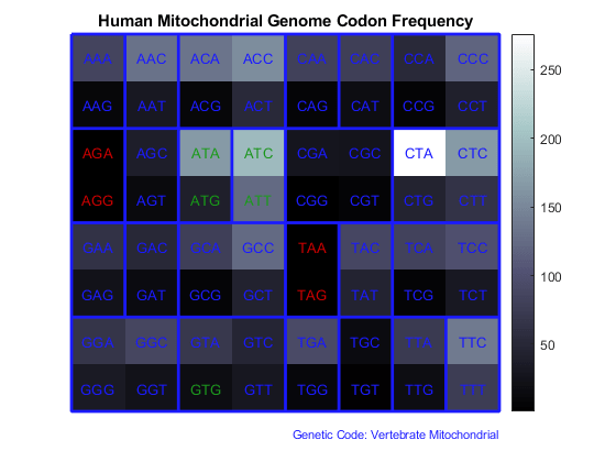
Use the figure option to the codoncount function to show a heat map with the codon frequency. Use the geneticcode option to overlay a grid on the figure that groups the synonymous codons according with the Vertebrate Mitochondrial genetic code. Observe the particular bias of Leucine (codons 'CTN').
figure
count = codoncount(allCDS,'figure',true,'geneticcode','Vertebrate Mitochondrial');
title('Human Mitochondrial Genome Codon Frequency')
close all
References
[1] Barrell, B.G., Bankier, A.T. and Drouin, J., "A different genetic code in human mitochondria", Nature, 282(5735):189-94, 1979.
You can also select a web site from the following list:
Americas
- América Latina (Español)
- Canada (English)
- United States (English)
Europe
- Belgium (English)
- Denmark (English)
- Deutschland (Deutsch)
- España (Español)
- Finland (English)
- France (Français)
- Ireland (English)
- Italia (Italiano)
- Luxembourg (English)
- Netherlands (English)
- Norway (English)
- Österreich (Deutsch)
- Portugal (English)
- Sweden (English)
- Switzerland
- United Kingdom (English)